Elastic Properties of Carbon Nanotube Reinforced Composites (top)
A polymer nanocomposite reinforced with single walled carbon nanotube is simulated using the LAMMPS
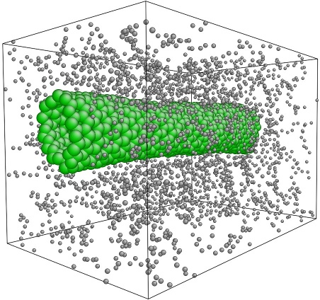
molecular dynamics code in order to obtain elastic properties. The simulation volume contains 10 polymer
chains that are 260 monomers long surrounding one central carbon nanotube containing 930 atoms. Due to
simulation restrictions, the atoms in the carbon nanotube are treated as a rigid body. The volume is
modeled as periodic in all directions.
 The rigid body restriction on the nanotube prevents calculation of longitudinal properties, therefore
displacements are only applied normal to the nanotube axis in order to obtain transverse properties.
The transverse properties are not directly affected by the nanotube, so a rigid nanotube is a reasonable
approximation. After each displacement is applied a time-averaged value of stress is calculated. LAMMPS
provides the stress contributions σijα from each atom as
The rigid body restriction on the nanotube prevents calculation of longitudinal properties, therefore
displacements are only applied normal to the nanotube axis in order to obtain transverse properties.
The transverse properties are not directly affected by the nanotube, so a rigid nanotube is a reasonable
approximation. After each displacement is applied a time-averaged value of stress is calculated. LAMMPS
provides the stress contributions σijα from each atom as
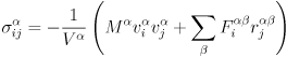 where superscript α corresponds to the atom, V is the atomic volume, vi and vj
are the velocity components in their respective directions, and Fiαβ and
rjαβ are the components of force and separation between atoms α
and β respectively. The stresses used to cerate the stress-strain curves are the average atomic
stresses across the volume of the MD model,
where superscript α corresponds to the atom, V is the atomic volume, vi and vj
are the velocity components in their respective directions, and Fiαβ and
rjαβ are the components of force and separation between atoms α
and β respectively. The stresses used to cerate the stress-strain curves are the average atomic
stresses across the volume of the MD model,
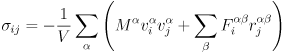 Here V is the simulation volume. These values of stress and strain are used to calculate Young's modulus
using Hooke's law.
Here V is the simulation volume. These values of stress and strain are used to calculate Young's modulus
using Hooke's law.
A uniform tensile strain is applied to the simulation volume normal to the axis of the nanotube. Strains are applied by resizing the simulation volume in the direction of the strain and rescaling the coordinates of the atoms to fit the new dimensions. Each iteration increases the length of the volume by 0.05 angstroms. The simulation is allowed to run until reaching 100% strain, meaning a displacement of 40 angstroms (4 nm) normal to the nanotube. After each iteration the system is allowed to equilibrate for 2,000 time steps, then the reported stresses for the next 1,000 time steps are averaged to produce a single value for stress at the current strain. Initially the response is linear-elastic and the stress-strain plots are used to calculate Young's modulus, according to Hooke's law. As the strain increases the polymer begins to fail and the stress-strain curves break down.
The simulation is repeated three times with different interface strengths between the polymer and the nanotube. The interface strength is based on the standard 12/6 Lennard-Jones potential,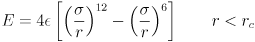 where ε is the depth of the potential well, σ is the distance at which the interparticle
potential is zero, and r is the distance between the particles. For this paper the interface strength is
adjusted using three different values of ε; εstd=0.00286 eV, εweak
=0.25εstd=0.000715 eV, and εstr=4εstd=0.01144 eV.
where ε is the depth of the potential well, σ is the distance at which the interparticle
potential is zero, and r is the distance between the particles. For this paper the interface strength is
adjusted using three different values of ε; εstd=0.00286 eV, εweak
=0.25εstd=0.000715 eV, and εstr=4εstd=0.01144 eV.
The stress-strain curves for the polymer-nanotube composite are included in Figure 2. The weakest interfaces experiences several partial failures under relatively low strain as the polymer separates and regroups along the nanotube. The polymer-nanotube interface is not strong enough to constrain the polymers, which mass together at one end of the nanotube and begin to separate from it as the strain increases. As the strain continues to increase the polymer separates completely from the nanotube and clusters in the gap between. With the standard strength interface the polymer continues to be evenly distributed along the nanotube, but it separates from the polymers in the periodic volumes on either side. Eventually only one polymer chain remains to hold the system together. The strong interface is very similar, except that the polymer chains remain even closer to the nanotube.
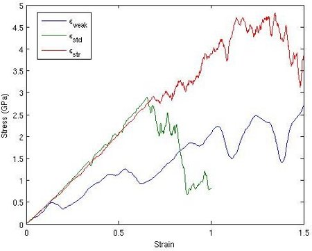 For relatively low strain the response of each nanocomposite is linear-elastic, therefore Young's modulus can
be calculated via Hooke's law. For the system with the weak interface three values of Young's modulus were
calculated, corresponding to the initial slope of the stress-strain curve and the slopes after the first two
partial failures. Averaging these three values results in an approximate Young's modulus of 3.67 GPa. The standard
strength interface and the strong interface were calculated using only the linear portion of the graph, resulting
in Young's moduli of 4.36 GPa and 4.22 GPa, respectively. The strong interface may have a lower elastic modulus
than the medium interface because the polymer chains are constrained too closely against the nanotube. This
prevents them from occupying the empty space and tying the simulation volumes together.
For relatively low strain the response of each nanocomposite is linear-elastic, therefore Young's modulus can
be calculated via Hooke's law. For the system with the weak interface three values of Young's modulus were
calculated, corresponding to the initial slope of the stress-strain curve and the slopes after the first two
partial failures. Averaging these three values results in an approximate Young's modulus of 3.67 GPa. The standard
strength interface and the strong interface were calculated using only the linear portion of the graph, resulting
in Young's moduli of 4.36 GPa and 4.22 GPa, respectively. The strong interface may have a lower elastic modulus
than the medium interface because the polymer chains are constrained too closely against the nanotube. This
prevents them from occupying the empty space and tying the simulation volumes together.
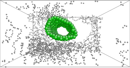
Initial state of the composite.
A uniform tensile strain is applied to the simulation volume normal to the axis of the nanotube. Strains are applied by resizing the simulation volume in the direction of the strain and rescaling the coordinates of the atoms to fit the new dimensions. Each iteration increases the length of the volume by 0.05 angstroms. The simulation is allowed to run until reaching 100% strain, meaning a displacement of 40 angstroms (4 nm) normal to the nanotube. After each iteration the system is allowed to equilibrate for 2,000 time steps, then the reported stresses for the next 1,000 time steps are averaged to produce a single value for stress at the current strain. Initially the response is linear-elastic and the stress-strain plots are used to calculate Young's modulus, according to Hooke's law. As the strain increases the polymer begins to fail and the stress-strain curves break down.
The simulation is repeated three times with different interface strengths between the polymer and the nanotube. The interface strength is based on the standard 12/6 Lennard-Jones potential,
The stress-strain curves for the polymer-nanotube composite are included in Figure 2. The weakest interfaces experiences several partial failures under relatively low strain as the polymer separates and regroups along the nanotube. The polymer-nanotube interface is not strong enough to constrain the polymers, which mass together at one end of the nanotube and begin to separate from it as the strain increases. As the strain continues to increase the polymer separates completely from the nanotube and clusters in the gap between. With the standard strength interface the polymer continues to be evenly distributed along the nanotube, but it separates from the polymers in the periodic volumes on either side. Eventually only one polymer chain remains to hold the system together. The strong interface is very similar, except that the polymer chains remain even closer to the nanotube.
Combined stress-strain curve for three values of ε.
Partial failure of composite with εweak.
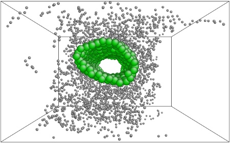
Failure mode for εstd.
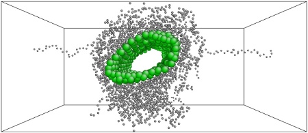
Failure mode for εstr.
References
- Frankland, SJV and Harik, VM and Odegard, GM and Brenner, DW and Gates, TS, The Stress-Strain Behavior of Polymer-Nanotube Composites from Molecular Dynamics Simulation. Composites Science and Technology, volume 63, pages 1655-1661, 2003.
Level-set Based Image Segmentation (top)
Go here to request the source code.
A level-set based image segmentation method based on a paper by Li et al. [1] has been implemented. The method eliminates the need for reinitialization by adding energy terms which force the level set to remain close to a signed distance function. The evolution equation is given by:
Two solution methods for this system of equations are compared. In the explicit solution time is discretized using the forward Euler method and solving for the next time step φn+1,
The explicit and semi-implicit methods produces very similar results, but the semi-implicit scheme has a significantly broader range of stable input parameters. The semi-implicit method was able to run stably with a Δτ of 60.0 for some problems, while the explicit method never ran stably with Δτ above 10.0. Larger time steps allowed the semi-implicit simulations to complete in a fraction of the time.
Two sample solutions are shown below, where blue lines are partially resolved zero-contours of the level set, and the final zero-contour is shown in red. The initial level set for both problems was defined as a rectangle near the edge of the image, where φ(x)=-6.0 for all x inside the level set and φ(x)=6.0 for all x outside the level set.
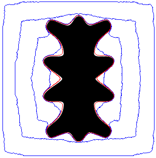
Explicit solution, 500 steps, λ=5.0, ν=7.0, Δτ=6.0, μ=0.04
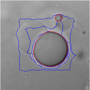
Implicit solution, 250 steps, λ=5.0, ν=3.0, Δτ=40.0, μ=0.01
References
- Li, C. and Xu, C. and Gui, C. and Fox, M., Level Set Evolution Without Re-initialization: A New Variational Formulation. IEEE Computer Society Conference on Computer Vision and Pattern Recognition, volume 1, pages 430-436, 2005.
Drucker-Prager Plasticity Model (top)
See the full pdf here, or go here to request the source code.
Pressure-dependent materials such as soil or concrete require advanced material models to predict yielding. A commonly used yield criterion is the two-invariant Mohr-Coulomb model, as described in (1.1), where the σi's correspond to principal stresses, c is the cohesion, and φ is the friction angle. On the π-plane, the Mohr-Coulomb yield surface is similar to a distorted Tresca yield surface with lower tensile strengths and higher compressive strengths. It is well suited to any porous or granular material in compression loading.
This paper will derive the Drucker-Prager smoothed approximation to the Mohr-Coulomb plasticity model, including a detailed account of the integration algorithm and numerical implementation. The Drucker-Prager yield surface and plastic potential are defined by
The Drucker-Prager material model is non-linear, so it is integrated with an iterative numerical scheme. In this paper a simple Newton-Raphson scheme is used in the material subroutine. Although the Drucker-Prager method only depends on two invariants, in this paper the more general three-invariant return mapping scheme is used. This is more difficult to implement, but can be applied to a broader range of material models. The method is a spectral method and therefore frame-invariant, and so can be easily applied to a broader range of material loading conditions. It requires the repeated calculation of eigenvalues and eigenvectors which can become computationally expensive in large models, but for the small numerical models presented here this is irrelevant.
Numeric Examples
Two numerical experiments are discussed. These are designed to test both the global loading iteration loop and the local material subroutine iteration loop. The common initial stress state is p0=-50 kPa and q=0 kPa, ie a hydrostatic state. Both experiments use vertical strain control and horizontal stress control. During loading, the vertical strain increment is Δε1 = -0.2% and the horizontal stress is kept constant. Both experiments stop at ε1 = -3%.Axisymmetric Loading
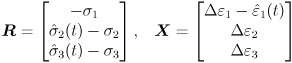
For the case of axisymmetric loading, a strain Δε is applied along the axis while the radial stresses σr are kept constant. In order to apply these complicated loading conditions, a global Newton-Raphson loop is implemented. The Newton-Raphson iteration scheme solves for the appropriate stresses and strains to meet the boundary conditions. We can write this as a residual vector R and a vector of unknowns X,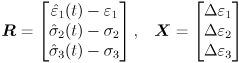
Under this loading, the Drucker-Prager is elastic for one loading step before going plastic. Once the material response is plastic, the material begins to soften.
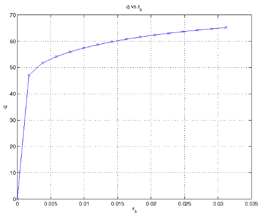
Axisymmetric loading, deviatoric stress vs. deviatoric strain.
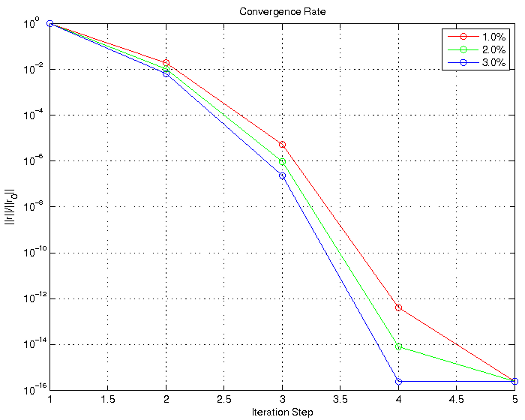
Axisymmetric loading convergence rates at several global loading points.
Plane Strain Loading
For the plane strain loading, a strain Δε is applied in the vertical (ε1) direction. The strain ε2 is maintained at zero, and only the stress is controlled in the third direction. Again, a global Newton-Raphson iteration scheme is used to apply these conditions. The same Newton-Raphson loop as in axisymmetric loading is used here, with a minor modification to control two strains instead of just one. Here we solve for the σ1 and σ2 values that correspond to the desired strain state before inverting the matrix.The results are similar to the case of axisymmetric loading. The additional strain constraint in the horizontal direction from plane strain causes higher stresses under loading.
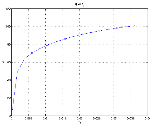
Plane strain loading, deviatoric stress vs. deviatoric strain.
Plane strain loading, volumetric strain vs. deviatoric strain.
References
- See the full paper here.
- R.I. Borja and J.E. Andrade. Critical state plasticity. Part VI: Meso-scale finite element simulation of strain localization in discrete granular materials. Computer Methods in Applied Mechanics and Engineering, 195(37-40):5115-5140, 2006.
- R.I. Borja, K.M. Sama, and P.F. Sanz. On the numerical integration of three-invariant elastoplastic constitutive models. Computer Methods in Applied Mechanics and Engineering, 192(910):1227-1258, 2003.
Galerkin and Petrov-Galerkin Stability Analysis (top)
See the full pdf here.
The advection-diffusion equation models situations where a substance is both transported and diffused through a medium. The one dimensional advection-diffusion equation for a particle concentration φ can be written
Solving the advection-diffusion equation using the standard Galerkin method can lead to oscillatory solutions caused by spatial numerical instabilities. The Petrov-Galerkin method is designed to alleviate these problems by essentially adding a viscous damping force. The implementation here is the Streamlined Upwind Petrov-Galerkin (SUPG) method in one dimension.
A specific model is implemented to show the differences between the Galerkin and Petrov-Galerkin methods. The simulation is a one meter segment of a long tube filled with solution. There is a steady state concentration of 5% at x=0 and 20% at x=1. The velocity u = 2.0 m/s and the diffusion coefficient v = 0.025 m2/s.
Finite Element Solutions
The Galerkin finite element discretization follows from the general form of the advection-diffusion equation. Using the test function w(x) and integrating over the domain,It can be shown that the stability of the Galerkin method depends on the Peclet number. If the Peclet number is less than one, then the Galerkin discrete solution approaches the exact solution. For Peclet numbers greater than one, the Galerkin discrete solution becomes oscillatory and the Petrov-Galerkin formulation is required. To illustrate this, the example problem in the introduction is run with several different Peclet numbers. To achieve the different Peclet numbers the resolution of the mesh is varied, using 10, 20, 50, and 100 elements.
The 10 and 20 element meshes result in Peclet numbers of 4.00 and 2.00, respectively. As shown below, the Galerkin method is unstable for these meshes and oscillates badly as x increases. Due to the proper choice of α, the Petrov-Galerkin method achieves the exact solution at the nodes, although the choice of linear shape functions limits the accuracy between nodes.
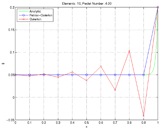
Stability at Peclet numbers greater than 1.0
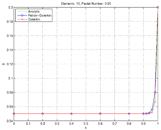
For the finer resolution meshes (50 and 100 elements), the Peclet numbers are 0.80 and 0.40, respectively. The Galerkin method is stable for these values, and compares favorably to the Petrov-Galerkin and analytic solutions.
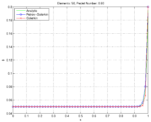
Stability at Peclet numbers less than 1.0
For all cases the Petrov-Galerkin calculates exact solutions at the nodes, due to the choice of α in one dimension. However, the finer meshes give a better resolution of the solution. For the Galerkin method, increasing mesh resolution results in more accurate values at the nodes.
SUPG Parameters
The choice of γ in the Petrov-Galerkin formulation plays a major role on the stability and accuracy of the solution. The γ term essentially adds an artificial viscosity to the solution to dampen oscillations. Incorrect choices of γ can lead to the solution being over-damped and inaccurate, or under-damped and oscillatory. In one dimension, γ can be calculated such that the solution is exact at the nodes.The solution with several values of γ has been plotted below. With low damping values the solution remains unstable, and with high values the solution is damped so much that the solution is no longer accurate.
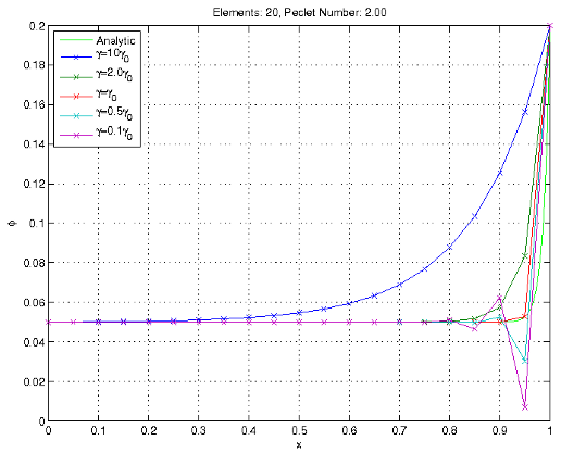
Different γ values, based off of the γ0 exact solution.
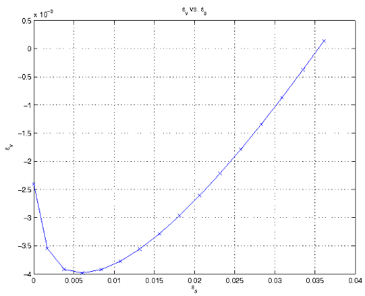
Non-uniform Mesh
The stability problems of the Galerkin formulation are spatial instabilities, caused by problems with the mesh. As shown in the previous Section, refining the uniform mesh eliminates the oscillations, at the cost of increased computational effort. Selectively refining the mesh around key areas allows the Galerkin solution to remain stable without unnecessary increased computation.In the example problem, the mesh is refined near the spike in concentration. The mesh on x=[0.9,1.0] is ten times finer than the mesh from x=[0.0,0.9]. The Peclet number is calculated based on the element length in the refined area. For this simple problem and simple non-uniform mesh, this Peclet number still results in exact solutions for the Petrov-Galerkin formulation.
Solutions for a simple non-uniform mesh.
For a more adaptively refined mesh, the calculation of the γ becomes more difficult, and it may not be possible to calculate a γ resulting in the exact solutions.